Excel template waterfall chart download

Participez au vote ☆☆☆☆☆★★★★★

Page suivante pour Télécharger

Excel template waterfall chart download

This article provides details of Excel template waterfall chart that you can download now.

Microsoft Excel software under a Windows environment is required to use this template

A waterfall graph displays the details of a variation of a bar graph.

For example, in a bar chart, you see a difference in value between the beginning and the end of the month.

However, you do not know what data has had a positive or negative effect on the overall result.

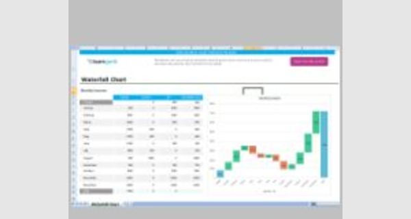
Let's put the data

To create a waterfall chart in Excel

Complex with previous versions of Excel (2013, 2010, etc.), the waterfall graph is created in a few clicks in the 2016 and 2019 versions.

It is useful for showing the cumulative effect of a series of positive and negative values between two points (departure and arrival). In a waterfall chart, the end point is the Total.

Start by entering your first value
Then enter all the "intermediate" data
End your list with the SUM function

These Excel templates waterfall chart work on all versions of Excel since 2007.

Examples of a ready-to-use spreadsheet: Download this table in Excel (.xls) format, and complete it with your specific information.

To be able to use these models correctly, you must first activate the macros at startup.

The file to download presents six Excel template waterfall chart

Microsoft Excel doesn’t offer a built-in waterfall chart, but a few extra columns of formulas added to your data can easily produce a cash flow waterfall chart. In a waterfall chart, the column begins with the previous month’s balance and travels up for positive amounts or down for negative amounts

To create the chart, you will add several quick columns to the original data set shown in Figure 1. First, add a balance column. Though this isn’t absolutely necessary, it makes the remaining formulas much easier. For 10 years, I built waterfall charts without this extra column and would beat my head against my desk as I tried to decode the formulas needed for the additional columns. The first row in the balance column is simply =Amount. Then each new row adds that month’s amount to the previous balance (=Previous Balance + Amount).

Now copy the month names to the next column. Then add four new columns: Invisible, Down, Up, and Grey. The Grey column is for the values that need to touch the x-axis. In this example, the first and last rows (Start and End) touch the baseline. The formula for the Grey column is =Balance.

The Up column needs to pull all of the positive amounts over. While you could use =IF(Amount>0,Amount,0), it’s quicker to use =MAX(0,Amount). This clever formula is handy for getting positive amounts. If the amount is greater than zero, then the amount “wins” in the MAX function. If the amount is negative, then the zero wins. It will hardly matter in this example, but the calculation time for MAX is a tiny bit faster than IF.

The Down column needs the absolute value of all negative amounts. While you might use =IF(Amount,0)*-1.

Formulating the Invisible Column

The Invisible column is the magic that allows the whole chart to work. The floating bars in the waterfall chart are going to be sitting on top of invisible columns. Follow along with this logic: If a month had negative cash flow, then the red column that will represent it on the chart is going to be traveling from the previous balance down to the current balance. That means that the invisible column needs to be the current month’s balance. The red column will sit on top of that value. But if a month’s cash flow is positive, then the top of the green column will have to reach up to the current balance, so the invisible column needs to be the previous month’s balance. The conceptual formula is =IF(Amount<0,Current Balance,Previous Balance). In Figure 2, the formula in H7 is =IF(E6><0,F6,F5).