
Excel template for trend-adjusted smoothing
Excel template for trend-adjusted smoothing
This article provides details of Excel template for trend-adjusted smoothing that you can download now.
Microsoft Excel software under a Windows environment is required to use this template
These Excel templates for trend-adjusted smoothing work on all versions of Excel since 2007.
Examples of a ready-to-use spreadsheet: Download this table in Excel (.xls) format, and complete it with your specific information.
To be able to use these models correctly, you must first activate the macros at startup.
To activate the smoothing methods dialog, launch XLSTAT, then select the XLSTAT / XLSTAT-Time / Smooth command, or click the equivalent button on the XLSTAT-Time toolbar.
When the button is clicked, the smoothing methods dialog box appears. You can then select the data on the Excel sheet.
The series to be analyzed corresponds to the studied series, Passenger data.
After selecting the data column, select the Holt-Winters method.
The Series Labels option is enabled because the first line of the series includes the name of the series
In the options tab, we choose the multiplicative seasonal model. Then, in order for the model parameters to be optimized (least squares criterion), we activate the optimized option for the three parameters. The period of the series is fixed at 12 because the traffic seems to know annual cycles (12 months).
Finally, in the validation tab, we put the value 12 because we want the last 12 months corresponding to the year 1960 not to be taken into account for the adjustment of the model, but that the forecasts are calculated for this period ( model validation).
Once you have clicked the OK button, the calculations start and the results are displayed.
The file to download presents tow Excel template for trend-adjusted smoothing
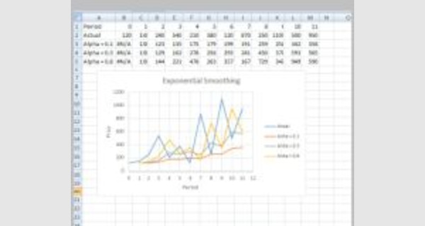
What is Exponential Smoothing?
The basic idea in exponential smoothing is that we take an average of our old estimate of some quantity, and some new information about that quantity. In exponential smoothing, we are assuming that there is no growth, no trend to the data. So every period, we are just making new estimates of the intercept.
Ft = α ∗ Dt−1 + (1 − α) ∗ Ft−1.
The new demand gives us another data point about what the intercept might be, and the old forecast is our old estimate of the intercept.
We can (and we are going to) use this idea to update estimates of other things, like a trend. Although the formula will look different, the idea is the same:
New Estimate = α · New information + (1 − α) · Old Estimate.
3 Forecasting with a Trend
When our demand has a trend, there are two main methods that we can use.
3.1 Linear Regression
I assume that you are all familiar with linear regression from your statistics classes. Basically, we assume that there is a linear relationship between one output (dependent) variable, Y , and the input (independent) variable, X. In our case, we will be looking at the independent variable as being time, t, and we think that demand is generally growing over time. We do a linear regression to get a formula like this: Y (t) = a + bt
For any time value, t, we put it into the equation, and get a straight-line forecast of the demand for that period. How well the data are approximated by the line is represented in the term R2 . R2 can be literally interpreted as the ”percentage of changes in Y that can be explained by changes in X. To do a linear regression in Excel, there are four ways you could do, presented in the order of the things I like the least to the way I think is the best. First, you could dust off your statistics book and type in the formulas from it. That sounds like a lot of work, and there are lots of opportunities to make a mistake when typing in those big formulas. But if you get it all in correctly, the spreadsheet will update automatically when you enter new data points.
Secondly, could also use the “Data Analysis ToolPak.” You should find that under “Tools — Data Analysis.” If it is not there, go to “Tools — Add-Ins.” In that dialog box, check the box by Analysis ToolPak. If that does not appear in the dialog box, you need to get out your CDs and install that part of Excel. After you go to “Tools — Data Analysis,” a dialog box comes up, where you tell it which cells are the X’s, and which are the Y’s. Tell it where to put the output, but be careful. If you put it on the sheet you are working on, the following 18 rows will get written over with the output.
In that output, you will want to look at where the “Intercept” row and the “Coefficient” column intersect. That is the intercept. The slope is the row below that, in the “X Variable” column, where it meets the “Coefficient” column. R-squared is in the second row of numbers, under “R Square.” One problem with this method is that when you add new data point to the spreadsheet, you have to go back up to “Tools — Data Analysis” every time to re-run the LR. The spreadsheet can’t update automatically. Thirdly, another way to get the intercept and slope is to create a graph of the data. Right click on the data line, and select “Add Trendline.” In that dialog box, add a linear trendline, and under “Options,” you can have the equation of the trendline displayed on the graph, and also R-squared. The trouble with doing the LR in the graph, is that you can’t make use of the numbers that appear in the graph in any calculations.
Finally, the best way to do the LR is to use the SLOPE and INTERCEPT functions. SLOPE(range of x value, range of y values) gives you the slope, and INTERCEPT(x values, y values) gives the intercept. To find out R-Squared, use RSQ(x values, y values).
Exponential Smoothing with a Trend
The only problem with Linear Regression is that it gives all the demand points equal weight when trying to fit a line. Really, we would like it to try hardest to fit the line to the most recent data points, and not worry quite so much about fitting the line to the oldest data points. Linear regression cannot do that.
However, we do remember that exponential smoothing had that type of behavior: give the most weight to the most recent. There is a way we can adapt exponential smoothing to work with a trend. (If you really want to be fancy, this is also known as Double Expnential Smoothing, or Holt’s Method.) We will define two terms:
St our estimate of the level at time t (kind of like an intercept, but not exactly).
Tt our estimate of the trend in period t, or the slope.
T AFt+1 = St + Tt.